

Introduction
The Purpose of Investment Portfolios
SS&C ALPS Advisors’ model portfolios are built to compound the hard-earned financial capital of individuals and households in diversified, multi-asset portfolios over the long-term. We believe strongly that the process of crafting an investment portfolio is directly related to an objective such as growing enough capital to spend freely in retirement, preserving capital to get through large expenditures or distributing income to use when an individual or household is no longer earning a salary. These outcomes of growing, preserving and distributing are objectives we use when building investment portfolios.
More specifically, investors have goals. Whether it be every day expenses, saving for something big, charitable giving, retirement income or leaving a legacy, goals should be considered explicitly in selecting the right portfolio. These financial goals can be viewed as liabilities to which the financial portfolio should be matched, with respect to both risk and return, to maximize the likelihood of achieving them.
Given extended bouts of market volatility, it’s understandable that some may not want to invest in financial markets. Over the long run, however, it is compelling. The theoretical framework for investing involves the concept of “risk premiums”1, which are returns that investors can expect over the long run. The risk premium originates from capitalism. In order to incentivize investors to send their savings to corporate or sovereign cash flow generators, the investments need to provide investors with an expected rate of return. That return can be fixed over some term, as in bonds, or it can be variable, as in stocks. In mature, dynamic and growing economies, this incentive structure typically leads to positive expected return on investment over the long run.
Multi-Asset Investing
In a world of multiple asset classes, we choose to build a multi-asset class portfolio. The reason being is that different asset classes have different useful characteristics and do not always move together, so using stocks, bonds and real assets together in a portfolio can smoothen the path toward achieving the investor’s objective. The key to compounding wealth over the long-term is not losing a bunch of wealth in any given year, and combining different asset classes in a diversified portfolio helps us achieve that goal.
If we were to set out to build a multi-asset portfolio, hypothetically it would make sense to purchase a portion of all the assets in the world – as the world grows, so does our portfolio. But of course, that is not possible, so we need some selection criteria. We could choose to own a handful of assets, and that seems plausible, but the problem here is that of under diversification – those handful of assets better work out. Ideally, we would like to own a lot of underlying investments so that if one does not work out, it will not take us off course from our objective. To that end we focus our attention on the universe of exchange-traded funds (ETFs).
|
The Model Portfolio Offering SS&C ALPS Advisors offers ETF-only, multi-manager model portfolios at the segment model level (e.g., the segment exposures within known asset classes) as well as multi-asset class, outcome-oriented portfolio solutions. With respect to the latter, both tactical and strategic tax-aware solutions are optimized specifically for use in qualified and taxable accounts, respectively. Tactical solutions implement model portfolios of 20 to 40 ETFs in a high turnover format, while the tax-aware strategic solutions implement model portfolios of 8 to 12 ETFs in a low turnover format. The focus of the higher turnover tactical solutions is to generate alpha in accounts that defer taxes, while the focus of the lower turnover strategic solutions is to capture the risk premia, or beta, associated with holding risk assets in a tax efficient way. The combination of both alpha and beta oriented strategies across taxable and tax deferred accounts encompasses another layer of diversification called strategy diversification which further enhances the risk-reward profile of the overall implementation. The multi-asset class portfolios are constructed from segment models to create an array of three objectives (Grow, Preserve, Distribute) and six risk targets (Protective, Conservative, Balanced, Moderately Aggressive, Aggressive, All Equity). This orientation is designed to meet investors in the accumulation, preservation and income life stages across the entire risk tolerance spectrum. Grow portfolios tend to run at full market risk within their risk target, Preserve portfolios prioritize low volatility, and Distribute portfolios prioritize income at below full market risk. |
 |
The remainder of this document provides critical background information and process description for the three main steps involved in our end-to-end model portfolio construction process:
- Security Selection
- Capital Markets Assumptions
- Portfolio Optimization
We only briefly cover Security Selection and Capital Markets Assumptions below as we have additional white papers that cover each these areas more deeply. We engage the reader here on the ideas and methodologies used in bringing all of the inputs together in the art of Portfolio Optimization.
Security Selection
Exchange-Traded Funds
The popularization of pooled investment vehicles started with mutual funds over 70 years ago, and have since evolved into lower cost, more transparent, tax-efficient ETFs. By pooling the interest of investors into a common portfolio, fund managers can create scaled, diversified exposures with tens or hundreds of underlying investments. ETFs have an edge over mutual funds because they are typically lower cost and have embedded tax advantages for growing capital. That is exactly the kind of low-cost diversification of investments we are looking for when building long-term, durable investment portfolios. Finding the best available ETFs can be a challenge, but we have streamlined this process with robust analysis enabled by technology. When building low-cost portfolios, we examine fund performance and utility across the entire playing field of ETFs – multiple managers, passive and active. We then identify the funds that express our investment views in the best and most cost-effective way.
Passive ETFs own assets with a remarkably simple investment rule. For stocks, that rule is to invest “passively” in all (or most) companies according to their size. In bonds, the rule is to invest in the debt of countries and companies according to the amount of their issuance. Passive ETFs have a lower cost, or expense ratio, because of how simple the investment process is to run. Active ETFs, however, invest in markets according to different rules, and those rules can be predefined or flexible over time as markets are confronted with new environments. Active ETFs have higher expense ratios because their investment process includes investment professionals attempting to identify better investments and avoid bad investments. While the average active fund manager has been shown to perform worse than passive investing after fees, there are some that do outperform and we leverage our internal tools to identify them.
Please refer to our Investment Due Diligence Process white paper for a deeper dive on how our investment team leverages technology and quantitative methods to identify ETFs with cost-effective exposures.
Capital Markets Assumptions
The Purpose of Research Team Views
The investment process is started with and continuously augmented by research team views, which are specific risk and return assumptions our Multi-Asset Research Team (the “MART”) formulates for covered asset class and asset class segments. We perform this exercise because asset classes and their relative segments move around in price and time, becoming more or less attractive in serving their role in a given portfolio objective.
A Yale professor named Robert Schiller calls this phenomenon “excess volatility” and has created a market valuation barometer called the Cyclically Adjusted Price-to-Earnings Ratio2 (or CAPE Ratio) to determine the relative attractiveness of the equity market over time. This ratio compares stock prices to their ten-year average earnings stream adjusted for inflation. When the CAPE Ratio is high relative to history, it means investors are assigning a “rich” valuation to the stock market, and when it is low, they are assigning a “cheap” valuation. Owning assets that are too rich poses a potential problem for portfolios because high valuations can be associated with higher risk and lower returns in the future. While the CAPE Ratio has been shown to work over long horizons, it has also misguided investors in the short and medium term. The reason for this is because the prices investors assign to stocks are also related to changes in expected cash flows, invested capital, growth rates and interest rates.
Equities
As a starting point, we utilize a building block model to formulate our expectation of return for stocks. Because the value of equity can be calculated as the present value of future dividends (or cash flows that will become dividends), we start with the dividend yield, add expected growth and a term for expected valuation change3, or the amount of return caused by investors reassigning rich or cheap prices to earnings:
Expected Equity Return = Dividend Yield + Growth + Valuation Change
Dividends and growth are observable and core to forming equity return expectations. Valuation change is more nuanced and is influenced by the mix of expected growth, profitability of reinvested capital and prevailing interest rates.
Please refer to our Equity Forecasting Framework white paper for a deeper dive on how our equities specialists make tactical recommendations among sectors and segments of the equity universe.
Fixed Income
Fortunately, it is a bit easier to forecast return expectations in bonds compared to stocks. For most fixed income asset class segments, a long enough investment horizon (3+ years) allows for the current yield to maturity to be a reasonable forecast of future returns. Using this as a starting point, we then focus on duration and credit spread risk as the main factors to refine the forecast. Losses in bonds are created by interest rate duration, or the bond’s price sensitivity to changes in interest rates, and spread duration, the bond’s price sensitivity to changes in its credit spread. We can incorporate these forecasts into a refined model for each fixed income asset class as follows:
Expected Return = Average Yield + (Interest Rate Duration * Δ Yield) + (Spread Duration * Δ Spread)
Please refer to our Fixed Income Framework white paper for a deeper dive on how our fixed income specialists leverage business cycle and monetary policy expectations analysis to forecast returns and make tactical recommendations among sectors and yield curve positioning.
Real Assets
Like equities, forecasting returns to real estate is a DCF exercise but with more stable cash flows because rents do not change often. As a result, they are sensitive to interest rates but with some embedded inflation protection, a feature that nominal bonds do not have. Given the stability in cash flows, valuation changes tend to be the best source of forecasting power in real estate investment trusts (REITs). Because of their bond-like characteristics, income yield from dividends provides a simple and effective starting point for forecasting long-term returns. The comparison of income yields to that of corporate bonds provides additional context with respect to the overall attractiveness of REITs, giving us a multi-asset perspective on the usefulness of real estate exposure in the investor portfolio.
Expected returns in commodities are related to supply and demand. More formally, the Theory of Storage4 posits that the expected returns in commodities are not constant over time but vary inversely with the level of inventories for the underlying commodity. When inventories are low, the risk of scarcity for consumers of the commodity rises, elevating spot prices and inducing higher expected price volatility in response to further supply or demand shocks. History shows metals and energy are powerful components to a strategic asset allocation, as the economic growth cycles that drive returns in equities have the potential to drive scarcity in metals and energy. Depending on the magnitude of economic downturns in nominal terms natural resources may play a key role in mitigating risk, particularly when the economic cycle includes an inflationary impulse.
Please refer to our Real Estate Investment Framework and Commodity Forecasting Framework white papers for a deeper dive on how our real asset specialists formulate capital market assumptions in their investment universe.
Portfolio Optimization
Data Preparation
Before building risk models for asset class segments used in portfolio optimization, we employ a procedure that backfills segment data where it may not exist in history. For all but a few of the oldest asset classes, historical data is limited by available pricing data. Using what is available is convenient and defensible but is of little use when considering how newer asset classes and segments may perform in more historical regimes (e.g., high inflation). To backfill newer asset class data through time, we utilize a standard statistical technique5 that extrapolates the observed relationships of newer asset class segments with a longer history time-series, generating history in line with how the newer segment may have behaved had it existed before it did.
|
Modern Portfolio Theory When building an investment portfolio, we attempt to optimize the tradeoff between expected return and expected risk. This idea originated from work of Harry Markowitz6 and others in the 1950’s and collectively is referred to as Modern Portfolio Theory (MPT). The mathematics of MPT was a breakthrough for its time, but a lesser known fact is how dependent the math is on the inputs – namely expected returns, risk and correlation. In fact, Modern Portfolio Theory assumes 100% confidence in these inputs. Consequently, our confidence in estimating these inputs should be a focus that drives our portfolio construction methodology. |
|
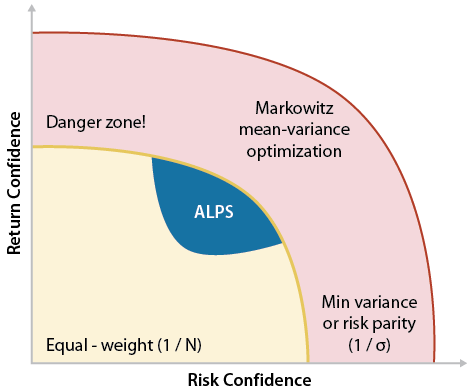
If we had little investment knowledge or confidence, we might equally weight asset classes and segments, otherwise known as the “naïve” investment strategy – a very simple approach. However, given our capital markets assumptions we understand that assets have relationships to the overall economy (growth and inflation), to their underlying cash flows (fundamentals and valuation) and to each other (correlation). Therefore, we can reasonably estimate how assets might perform in the future and, subsequently, would want to identify the mix of assets that provide a portfolio with the best estimated reward per unit of risk for a given investment objective.
Problems arise when we become too confident. We do not know the future exactly. To accommodate for this obvious detail, we take steps to consider “estimation error” - how closely the historical in-sample asset behaviors (returns, volatility and correlation) resemble the future out-of-sample behaviors we are trying to predict. We explicitly consider the possibility that our expectations of the future are wrong because financial markets are “wicked”. In his book Range7, David Epstein discusses the difference between kind and wicked domains:
[In] “kind” learning environments. Patterns repeat over and over, and feedback is extremely accurate and usually very rapid. In golf or chess, a ball or piece is moved according to rules and within defined boundaries, a consequence is quickly apparent, and similar challenges occur repeatedly…

In wicked domains, the rules of the game are often unclear or incomplete, there may or may not be repetitive patterns and they may not be obvious, and feedback is often delayed, inaccurate, or both. In the most devilishly wicked learning environments, experience will reinforce the exact wrong lessons. [emphasis added]
Addressing Estimation Error
The most common way to estimate return and risk of asset classes and asset class segments is to compute the mean, variance and covariance of their historical returns. This seems practical as we can summarize how assets have behaved given their available pricing history. However, creating such a summary of behavior would implicitly inform a portfolio optimization that the forthcoming return, risk and correlation of assets will look like a statistically manufactured composite of their available history.
|
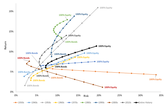
To illustrate, in the associated figure we’ve plotted the realized efficient frontiers of stock and bond blended portfolios for each decade back to 1930. We have also plotted the efficient frontier built from the entire history in black. Importantly, the historical composite lies far away from over half of the realized decades. Furthermore, using an efficient frontier from the previous decade to predict the following decade in most cases would lead the portfolio astray. This is a clear visualization of the estimation error associated with leaning too heavily on contemporary data or long-term statistical composites to generate estimates of future turn. |
|
There are at least three ways of dealing with estimation error in portfolio optimization. The associated table describes each method and its respective mechanism and outcome. We make use of all three methods in an attempt to import estimation error into the portfolios.
| Method | Mechanism | Outcome |
| Constraints | Add explicit hard or soft asset weight constraints in the optimization | Most popular method, but can be costly when constraints prevent portfolios that would have been better when estimate errors were low |
| Resampling | Add Monte-Carlo style random draws of perturbations of the return and risk inputs, then solve for average of optimal portfolios for each set of inputs | Communicates optimal asset weights as ranges rather than point values, works very well for asset allocation |
| Bayesian Methods (e.g. Black-Litterman) |
Condition expectations not only on historical data, but other “prior beliefs”, such as the cost of being wrong | Wrongness costs are highest for extreme outlier estimates |
Bayesian Portfolio Management
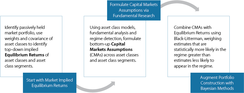
The associated graphic provides an overview of the steps involved in refining our capital market assumptions prior to portfolio optimization.
|
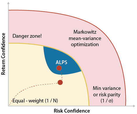
For tactical segment model construction, where our medium-term capital markets assumptions are used in an attempt to generate alpha, our portfolio construction process reflects an extension of the Black-Litterman8 method. This is a Bayesian updating process of inputs that precedes Markowitz’s portfolio optimization. Specifically, the Black-Litterman process considers the likelihood our capital market assumptions are correct, giving more weight to our expectations as they take on a greater likelihood of manifesting themselves in the return distribution of the current regime. As our expectations drift further from the returns distribution of the current regime, more weight is given to the equilibrium returns, or the returns extracted directly from an asset class’s segment-level capitalization weights and covariance matrix. Building directly to these equilibrium returns can be thought of as building a benchmark portfolio. In other words, prior to portfolio optimization, we are blending our own capital market assumptions with that of the benchmark portfolio in a way that prioritizes specific capital market assumptions when they do not look like a statistical outlier. This process navigates our portfolio up in the risk-return confidence graphic, thoughtfully building incremental confidence in our return expectations without assuming 100% confidence. |
|
Tail- and Regime-Aware Portfolios
When constructing strategic models and the multi-asset class objective-oriented portfolio solutions from our tactical segment models, we employ resampling as a way to import estimation error and guide the portfolio toward the best risk-reward outcome given the expected market regime over the long-term investment horizon. Resampling is an exercise in simulation, calculating thousands of paths asset classes could take given what we know of their historical return distributions. We use these simulations as inputs into the mean-variance portfolio optimization process to effectively identify a range of optimal weights for assets in a given investment objective and risk target. This directly imports noise into our optimal portfolios, increasing the durability of our estimates and our portfolios.
As negative tail events manifest themselves explicitly as observations in these simulations, our final portfolios are enhanced with a tail-awareness that we expect to attenuate downside risk. Furthermore, as our regime detection and filtering efforts produce distributions that are more in line with the realized market regime, our portfolios are expected to be enhanced with a regime-awareness that helps to direct asset and segment model weights to the most likely realized efficient frontier over the investment horizon. The promotion of tail- and regime-awareness are key aspects to our portfolio construction process which we believe differentiates it from the typical exercise of using full sample averages, variance and covariance of asset returns.
Finally, constraints are used in the formation of both segment models and multi-asset class portfolios as necessary. These might include hard asset constraints to satisfy portfolio characteristics (e.g., duration) or objectives (e.g., yield), as well as any overrides our co-CIOs would make to enhance the forward-looking risk-reward of a given portfolio.
Portfolio Surveillance
The information sets created by the Bayesian updating of our research team views are integrated into our portfolio management process via an internal web application called ModelLab. Daily updates of ex-post performance, tracking error, attribution and ex-ante risk estimates are provided via tables and visualization to keep the Multi-Asset Research Team abreast of real-time performance, risks and opportunities. We view the portfolio construction process as a living and breathing practice that requires constant evolution and enhancing, so the feedback mechanism on performance of views and optimization methods are a critical part of the differentiated model portfolio offering.
References

1    Damodaran, Aswath. 2016. “Equity Risk Premiums (ERP): Determinants, Estimation and Implications—The 2016 Edition” (5 March): https://ssrn. com/abstract=2742186.

2    Campbell, John H., and Robert J. Shiller. 1988. “Stock Prices, Earnings, and Expected Dividends.” Journal of Finance, vol. 43, no. 3 (July): 661–676.

3    Jarrod W. Wilcox (1984) The P/B-ROE Valuation Model, Financial Analysts Journal, 40:1, 58-66, DOI: 10.2469/faj.v40.n1.58

4    Gorton, Gary B., Hayashi, Fumio and Rouwenhorst, K., (2013), The Fundamentals of Commodity Futures Returns, Review of Finance, 17, issue 1, p. 35-105.

5    Stambaugh, R. F. (1997). Analyzing Investments Whose Histories Differ in Length. Journal of Financial Economics, 45 (3), 285-331.

6    Markowitz, H. (1952) Portfolio Selection. The Journal of Finance, 7, 77-91.

7    Epstein, David. Why Generalists Triumph in a Specialized World, 2019.

8    Global Portfolio Optimization (Black, Fischer, Litterman, Robert, 1992).

AAI001058